By Barthold Pieters – Data Scientist
Recently, someone thought it interesting to demonstrate customers the potential of AIOps: that is, AI powered IT operations. Think smart IT ticketing, streamlined incident management, and predictive scaling of resources. So what better way than asking InfoFarm to develop an interactive app showing just that?
At this very moment, a Python Dash application is in full development, whose purpose is to visualize improvements on current business processes using both historic and live data. Among them: automated up- and downscaling of resources, which will be the focus of this post.
So, what exactly is automated up- and downscaling?
Consider a medium-sized online retailer handling multiple users 24/7. Presumably there are periods of high and low traffic during day- and night time respectively, the store runs a server capable enough to handle the fluctuating traffic. So far so good. But wait! Weekly back-ups are known to notoriously put a strain on the server’s capacity. Oh my, what will the retailer do?

Apparently, employing additional servers manually is the preferred way to deal with increased load. Nothing the retailer cannot handle! However, what with sales causing even greater loads? And idle servers during subsequent low traffic? Is this strategy still cost-efficient? Not to mention perfectly automatable?
Meet predictive scaling: automated acquisition and release of cloud computing power according to predicted load, i.e. better performance for less costs. Profit!
Having received 200Gb of data consisting of Jira tickets, Apache logs and DataDog server metrics, our Farmers were excited to dive into the realm of AIOps. First off, an exemplary Data Scientist starts with exploring data. Let’s take a look at some server CPU loads over time.
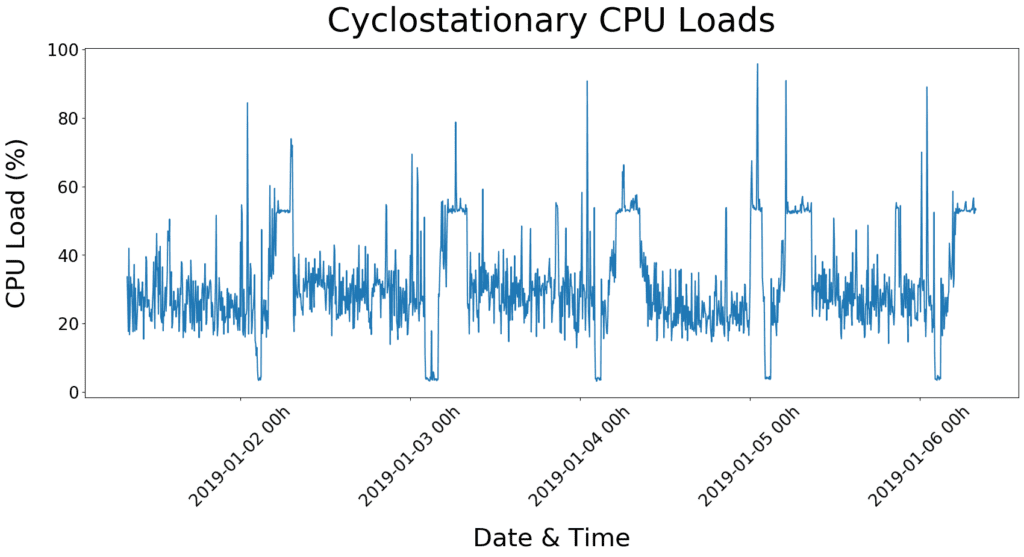
At first glance, the data display a non-stationary—but stable seasonal (i.e. cyclostationary)—pattern. In other words, statistical parameters such as average and variance are time-dependent within daily cycles but remain stable between cycles.
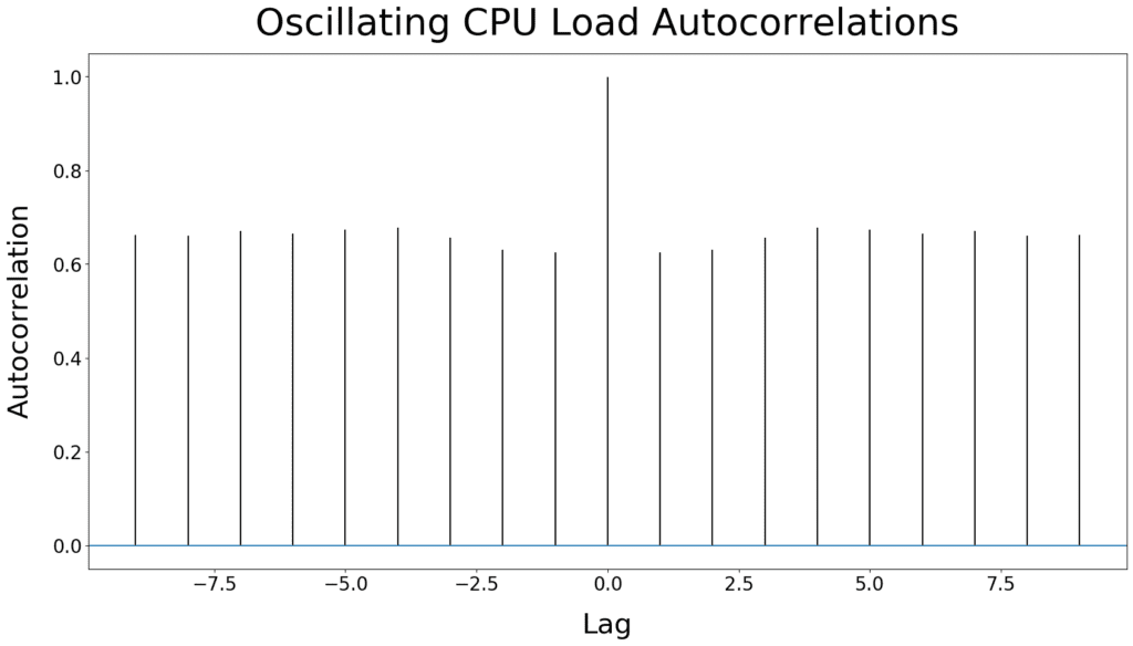
We checked this assumption using the Augmented Dickey-Fuller test and results indicate data to be non-stationary (i.e. test statistic=-2.6512 and p-value=0.0829, with H0=data are non-stationary and H1=data are stationary). Combined with the associated autocorrelation plot clearly showing an oscillation, which is indicative of a seasonal series, we concluded CPU loads in addition to be seasonal.
Since the data are seasonal, we continued modelling the data using the Seasonal AutoRegressive Integrated Moving-Average (SARIMA). SARIMA basically specifies the output variable depends on its own previous values through a linear model, while also stating the regression error is a linear combination of error term values occurring contemporaneously and at various times in the past. (If that didn’t make any sense at all, just continue.)
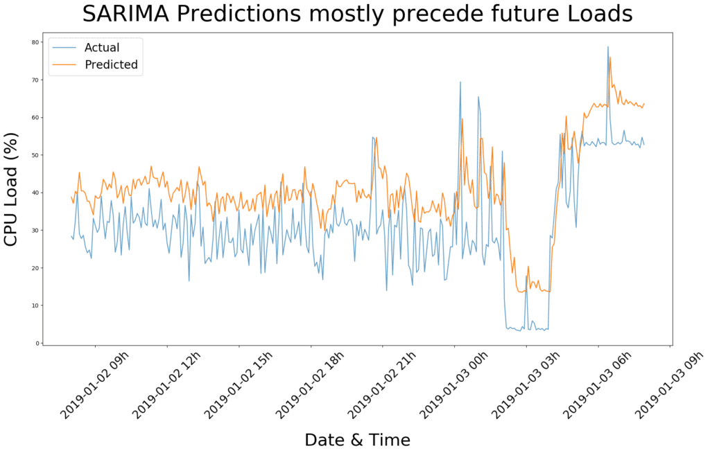
Essentially, we apply SARIMA to predict future CPU loads using past loads, with the goal to save costs by scaling CPU resources accordingly. A figure comparing predicted versus actual CPU loads for one day is shown below. Fairly good results were obtained within the first few runs (i.e. root-mean-square error=12.9), where predicted values (cf. orange trace) stay ahead of the actual observations (cf. blue trace) in most cases.
Although predictions were okay-ish, SARIMA scored less than satisfactory in the speed department. On average it took more than 33 seconds to generate upcoming predictions, which is too slow for live extrapolation. We needed a more efficient function. Something fast with similar accuracy. Then somebody of us mumbled “What about exponential smoothing?”. ¯_(ツ)_/¯
Like SARIMA, exponential smoothing (in our case Triple Exponential Smoothing, also known as Holt-Winters method) utilizes past CPU loads to make predictions about future loads. The difference is in the weighting of past observations. Namely, older observations are assigned smaller weights, whereas more recent observations receive higher importance in predicting subsequent loads.
Armed with our state-of-the-art knowledge and the latest statsmodels package, we unleased exponential smoothing on the CPU metrics. First try:
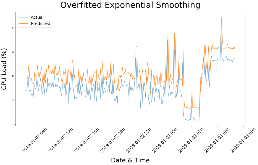
Pretty neat, considering it took less than a second to compute. However, we clearly overfitted the data by assigning too much weight on recent observations (notice the orange trace is simply a copy of the blue trace shifted in time?). This is just a matter of including more past data points to smooth out the seasonal pattern, which should be easy to implement. So, without further ado, let’s apply some smoothing!
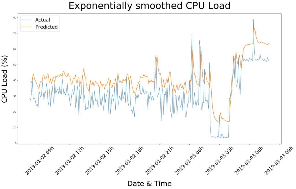
Ta-da! Not only do the predicted values fluctuate less than with SARIMA, the root-mean-square error of 11.11 is also slightly lower, indicating a more accurate predictive model. It is not perfect yet, but combined with the faster performance, we solemnly appoint exponential smoothing the clear winner for our purposes in predictive scaling.
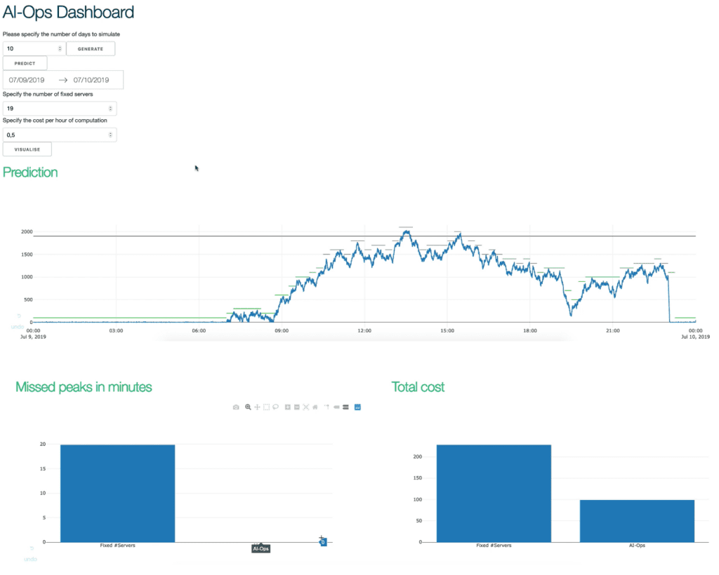
Below is a reduced view of our dashboard with an optimized exponential smoothing function. Next to peak handling performance and cost saving graphs, you can clearly see resources are scaled efficiently (cf. green traces) to the actual CPU loads (cf. blue trace), whereas a setup with fixed resources (cf. black trace) stays stationary. Just look at the cost savings!
And with that, we wrap up our post on AIOps and predictive scaling. Thank you for reading if you made it this far; hope you enjoyed it!