ETL on AWS – Time to face, a real-life case!

Hi, I’m jasper callaerts! You’ll probably remember me from the previous blog about etl on aws. In that blog we learned all about aws glue and its components. We learned why and when we should (not) use it, but we don’t exactly know how to use it. That’s what we will learn today! The goal of this second blog about etl on aws is to apply the theory that we’ve learned in the previous blog and experience what it’s like to build an etl pipeline and how glue interacts with other aws services.

Let’s build our own ETL pipeline!

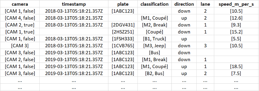
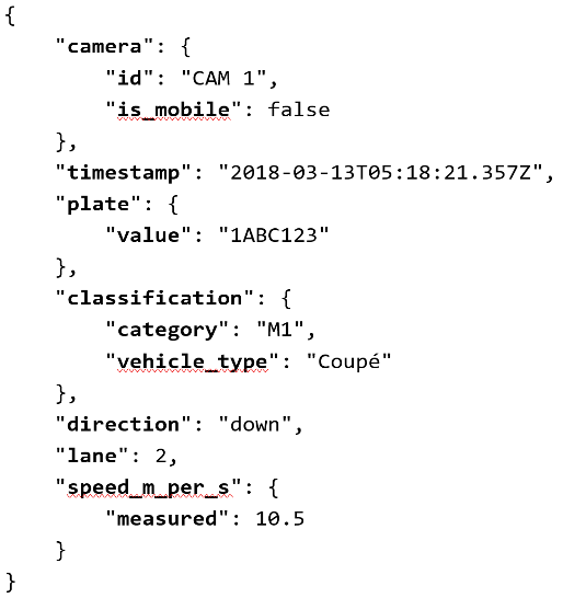
In this section we will build our own (simplified, high level) ETL pipeline, based on a real case that I implemented. For this we take the example of traffic cameras. These cameras register every vehicle that passes by. Through an ingestion API (which we learned all about in this blog the raw data from these cameras comes into our data lake. Below, you can see a simplified example of a single record of data coming in, as a JSON string. The data comes into our landing bucket in this format. Below the JSON string, there are more example records, shown in a table. You can see that some of the records have missing values. Later in this blog, we will learn how we approach the situation of missing data.

Data storage

Glue can read data from a database or an S3 bucket. In our example, we will use S3 as our main storage service. We have multiple buckets (landing – raw – accepted – master) in order to create our data lake, as we learned in this blog. The data shown above comes into the landing bucket in JSON format.

We will perform 3 separate ETL steps to move the data through the different buckets. In the raw bucket we will store the data in the same way as in the landing bucket, but with different partitioning. We will repartition the data by year/month/day, based on the timestamp that each record is ingested in the raw bucket. This is typically done by a Lambda function. In the accepted bucket, we will only store the records that were approved in our second ETL and repartition them, this time based on the timestamps we find in the records themselves. Usually, we store the data in PARQUET format instead of JSON in this accepted layer. In the master bucket, we store the output of the third ETL, which is usually a transformed/aggregated version of the data.

Data catalog

Before we can transform the data using our Glue Jobs, we must create the data catalog. Namely, we need a Glue Table, containing the structure of the data, for reading the input data in a Glue Job. Also for querying the output data of the Job, we need a table of this data. Since we will only use Glue for the second and third ETL job, we only need to catalog the data in the raw, accepted and master buckets.

So, we must create a Glue Crawler for each of the three buckets. The crawlers will catalog all files in the specified S3 buckets and prefixes. All the files should have the same schema. In Glue crawler terminology, the file format is known as a classifier. The crawler identifies the most common classifiers automatically including CSV, JSON and PARQUET.

The crawlers automatically create Glue Tables and add them to a Glue Database (or it asks you to create one during setup), containing metadata. Glue tables don’t contain the data but only the instructions on how to access the data.

So for this example we will have 3 crawlers, 1 database and 3 crawlers.

Data transformation

Now that we have our data in the S3 landing bucket and we also have our crawlers and tables set up, we can start to create the core of our ETL pipeline: the scripts.

Landing to Raw

As we already mentioned above, the first ETL step is copying the data from landing to raw and partitioning this data by year/month/day based on the ingestion timestamp. This ingestion timestamp is not necessarily the same as the timestamp in the record. Since this is not a heavy task, it is perfect for a Lambda function. This means that the structure in the raw bucket will be the following:

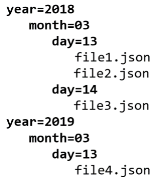
You can see that there is also a file in the partition ‘year=2018/month=03/day=14’, even though there is no record in our example with that timestamp. This shows the difference between the ingestion timestamp and the record timestamp, and it shows that it is possible that the data ingestion can be late.

Raw to Accepted

This is a very important step in the whole ETL process. Here, the goal is to filter out the bad records, to put more structure into the data (e.g. by flattening the data or enforcing a timestamp format), to enrich the data (e.g. joining with another table) and to repartition it by year/month/day of the record timestamp. In this step we want to keep as much of the data as possible, so that it can be used for any purpose in the next ETL step.

For example, when we look at our data, we immediately see that not all records contain all the data. The first record has no classification, the second record has no number plate, the fourth record has no timestamp, etc. For some fields this doesn’t have to be a problem (e.g. classification, speed, …), but for the timestamp field for example, this is problematic, since we rely on that field to partition the data. For this example, we take the camera_id, the timestamp and the plate_value as our mandatory fields, which must be present in the data. When this is not the case, the record is simply thrown away.

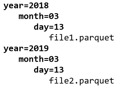
After our second ETL job, the data will be partitioned like this:

And will probably look something like this:

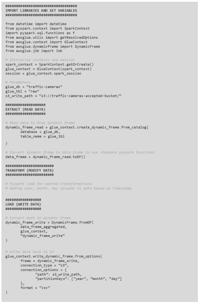
You can see that the columns are flattened, that null values are filled in the empty places and that we removed 2 records from the data (record 2 and 4) because of a missing plate_value and a missing timestamp.

Below is a code snippet for this ETL Glue Job:

Accepted to Master

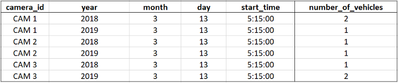
In this last step we will transform the data by aggregating it, to gain specific insights. There are many possibilities in this step, and so there can be many master buckets. The idea is that for each specific requirement, you only have to start from the accepted data bucket and transform the data according to the requested need.

For example, we can count the number of vehicles, per camera, every 5 minutes (as shown in the example below). It is also possible to compute the average speed of the vehicles, per camera, per vehicle type, for each day.

This data can then be queried via Amazon Athena, after being crawled by the Glue Crawler. It is also possible to visualize this data in Amazon QuickSight.

Data Orchestration

All these different steps now have to fit together and be executed in a specific order. Glue offers a functionality for this, called Glue Workflows. With this service, you can schedule each Glue functionality and make a chain of events. This is very handy when you’re only using Glue functionalities in your pipeline, but often this is not the case. So that’s why I rather use AWS Step Functions for orchestrating everything.

What have we learned today?

I hope you have learned how AWS Glue is a key service in your serverless platform, when you should use it and how you can easily integrate it in your architecture. Of course, as with every technology, you will still be frustrated a lot and will find yourself questioning your life choices when you face the error below for the six millionth time, but once you know your way inside the Glue Ecosystem, you won’t stop using it!